Introduction: The GenAI Age — Creating Instead of Curating

Generative AI (GenAI) is transforming the landscape of technology, powering applications which can generate audio, art, or photorealistic images. We have seen a recent trend of Ghibli images being famous throughout the world, as millions of users use ChatGPT DALL-E to generate cartoon-like images by uploading their original images. Although the advanced image generation models use Diffusion techniques instead of Variational Autoencoders, it is interesting to understand how it all started. Generation of any new article, music, or drawing is particularly challenging for humans, as the human mind works best for classification (e.g. distinguishing between two or more objects). The same is the challenge for machines, while classification tasks are comparatively easy for computational engines, generation requires more intricate techniques and, of course, lots of computational power. Images are high-dimensional representations of the real world scene, and the generation of new images would not be possible if the machine doesn’t understand how to deal with the same. Variational Autoencoders, a foundational model, are thus introduced to solve this problem.

What is a Variational Auto Encoder (VAE)?

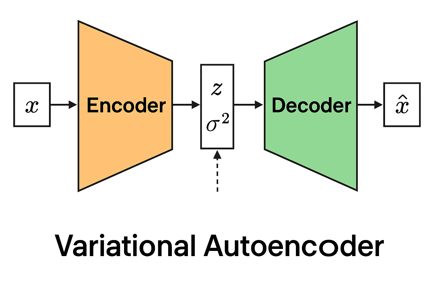
A VAE learns to encode real-world data (e.g. images, text, speech) into a compressed latent space before reconstructing or generating new data points from this space.

How does it work?

• Encoder: Projects input x into a lower-dimensional latent variable z, which represents the original input.

• Latent Space: Latent space is a lower-dimensional, structured representation learned, where complex data, such as images or sounds, are encoded as abstract, meaningful features that capture the underlying variations in the data.

• Decoder: Regenerates data from sampled latent representations, which means the network can create new similar data, not just reconstruct the input.

$$\text{Dimension of Input Variable:} \quad x \in \mathbb{R}^D$$

$$\text{Dimension of Latent Variable:} \quad z \in \mathbb{R}^K$$

$$\text{where} \quad K <

Image by EugenioTL - Own work, CC BY-SA 4.0, https://commons.wikimedia.org/w/index.php?curid=107231101

Math Behind the Magic

The core of Variational Autoencoders (VAEs) is the optimisation of the Evidence Lower Bound (ELBO), which balances two goals:

• Accurately reconstructing data from the latent space.

• Ensuring the latent encodings follow a standard, well-behaved distribution (typically Gaussian).

$$\mathcal{L}(x_n, z_n, \psi, \theta^x) = -\log p(x_n | z_n, \theta^x) + D_{KL}\big( q(z_n|x_n, \psi) \;\|\; p(z_n) \big)$$

where:

$$p(x_n | z_n, \theta^x) \; \text{is the likelihood term for reconstructing the data}$$

$$q(z_n|x_n, \psi) \; \text{is the approximate posterior from the encoder}$$

$$p(z_n) \; \text{is the prior over latent variables (usually a standard normal).}$$

$$D_{KL}\big( q(z_n|x_n, \psi) \;\|\; p(z_n) \big) \; \text{is the Kullback-Leibler (KL) divergence, regularizing the latent space.}$$

The reparameterization trick allows gradients to flow through stochastic nodes, making training possible (crucial for GenAI scalability).

Core Intuition

So far, we have defined the loss function of the Variational Autoencoder for training the model to reconstruct (or generate) new data samples. Minimising the loss would lead to the output of the decoder being close to the actual image input. Using techniques such as Backpropagation and Stochastic Gradient Descent, we compute the gradient of the loss function with respect to all network parameters by applying the chain rule backwards through the network layers — from the decoder output, through the latent space, back to the encoder input. Then, we update network parameters to minimise the loss function.

Complete ELBO Loss is a combination of two parts:

• Reconstruction Loss: Measures how well the decoder can recreate the original input from the latent representation, typically using mean squared error or binary cross-entropy.

• KL Divergence Loss: Regularises the encoder’s latent distribution to stay close to a standard normal distribution, ensuring the latent space remains well-structured and enabling smooth generation.

Inference Phase: From Latent Code to New Data

After training is completed, we remove the encoder block from the scenario and now rely on the decoder block to generate new data samples (e.g. images). Unlike training (which encodes real data into latent space), inference starts from the latent space and generates entirely new outputs.

VAE inference follows a straightforward three-step process:

• Sample from the prior: Draw a random latent code from the learned prior distribution (typically standard normal).

$$z’ \sim p(z|\theta^z)$$

• Compute decoder parameters: Use the decoder network to map the latent code to output distribution parameters.

$$\hat{\theta}^x = f(z’; \theta^x)$$

• Generate the output: Sample the final output from the parameterised distribution.

$$x \sim p(x|\hat{\theta}_x)$$

The ELBO Reparameterization: Making VAE Training Possible

While the ELBO objective we discussed earlier provides the conceptual framework for VAE training, there’s a critical mathematical challenge: how do you backpropagate through random sampling? The answer lies in an elegant mathematical trick called the reparameterization trick.

$$z_n = h(x_n; \psi)\mu + \epsilon_n h(x_n; \psi)\sigma$$

Instead of sampling z directly from the encoder’s output distribution, we express it as above.

where:

$$h(x_n; \psi)\mu \; \text{and} \; h(x_n; \psi)\sigma \; \text{are the mean and standard deviation output by the encoder}$$

$$\epsilon_n \sim \mathcal{N}(0,1) \; \text{is noise sampled from a standard normal distribution}$$

This reparameterization transforms the optimisation problem into

$$\arg\min_{\psi,\theta^x} \mathbb{E}{x_n,\epsilon_n} \;\mathcal{N}(x_n|f(z_n; \theta^x)\mu, f(z_n; \theta^x)\sigma) + D{KL}(q(z_n|x_n, \psi), \mathcal{N}(z_n|0,1))$$

The brilliant insight is that gradients can now flow through the deterministic functions

$$h(x_n; \psi)\mu \; \text{and} \; h(x_n; \psi)\sigma$$

$$\text{while the randomness is isolated in} \; \epsilon_n$$

Source: Puchalski, Andrzej & Komorska, Iwona. (2023). Generative modelling of vibration signals in machine maintenance. Eksploatacja i Niezawodnosc - Maintenance and Reliability. 25. 10.17531/ein/173488.

Closed Form KL Divergence

KL divergence can be computed analytically when dealing with Gaussian distributions:

$$D_{KL}(q(z_n|x_n, \psi), \mathcal{N}(0,1)) \propto -\log h(x_n; \psi)\sigma + \frac{1}{2}h(x_n; \psi)\sigma^2 + \frac{1}{2}h(x_n; \psi)_\mu^2$$

Without the reparameterization trick, VAE training would be impossible. It’s the mathematical bridge that allows us to:

• Maintain the probabilistic nature of the latent space

• Enable gradient-based optimisation

• Scale VAE training to complex, high-dimensional data

Simplified Loss

While the full VAE formulation with probabilistic outputs is mathematically elegant, practitioners often use a simplified version that’s easier to implement and train while maintaining most of the benefits.

Instead of the full probabilistic framework where we sample from the decoder output distribution, we can directly use the mean as our reconstruction.

$$\hat{x} = f(z_n; \theta^x)_\mu$$

This omits the variance term, transforming our complex probabilistic generation into a straightforward deterministic reconstruction.

Simplified Loss Function

$$\arg\min_{\psi,\theta^x} \mathbb{E}{x_n,z_n} \sum{d=1}^{D} (x_{n,d} - f(z_n; \theta^x)d)^2 + \sum_{k=1}^{K} \left[-\log h(x_n; \psi){\sigma_k} + \frac{1}{2}h(x_n; \psi){\sigma_k}^2 + \frac{1}{2}h(x_n; \psi)_{\mu_k}^2\right]$$

where:

• The first term is a simple mean squared error (MSE) between the input and the reconstruction.

• The second term is the analytical KL divergence regularising the latent space.

Why this works in practice

This simplified approach offers several advantages:

• Computational Efficiency: No need to sample from the decoder distribution during training, reducing computational overhead.

• Implementation Simplicity: The loss becomes a straightforward combination of reconstruction error and KL regularisation, much easier to code and debug.

• Stable Training: Removing the stochastic sampling from the decoder output often leads to more stable gradients and faster convergence.

• Retained Generative Power: The latent space still maintains its probabilistic structure through the encoder, preserving the model’s ability to generate diverse samples

VAE Algorithm

We have covered the most important mathematical aspects in the past sections; now, let’s explore how we can implement this programatically.

Data:
    •    D: Dataset
    •    q_φ(z|x): Inference model
    •    p_θ(x, z): Generative model
Result:
    •    θ, φ: Learned parameters
Algorithm:
(θ, φ) ← Initialize parameters
while SGD not converged do
    M ~ D (Random minibatch of data)

    ε ~ p(ε) (Random noise for every datapoint in M)
    Compute L_θ,φ(M, ε) and its gradients ∇_θ,φ L_θ,φ(M, ε)
    Update θ and φ using SGD optimizer
end

Source: D. P. Kingma and M. Welling, “An Introduction to Variational Autoencoders,” FNT in Machine Learning, vol. 12, no. 4, pp. 307–392, 2019, doi: 10.1561/2200000056.

Conclusion

Variational Autoencoders represent far more than just another neural network architecture—they embody a fundamental shift in how machines understand and create. By learning to compress the essence of data into structured latent spaces and probabilistically generate new samples, VAEs laid the mathematical groundwork for the entire GenAI revolution we’re witnessing today. While modern systems like ChatGPT, DALL-E, and Stable Diffusion have moved toward diffusion models and transformers for their impressive results, they all build upon the core insights pioneered by VAEs: the power of latent space representations, the importance of probabilistic generation, and the elegant mathematics of variational inference.

Key Takeaways

• VAEs solved the fundamental challenge of teaching machines to generate rather than just classify.

• The ELBO objective and reparameterization trick remain essential concepts in modern generative modelling.

• Probabilistic latent spaces enable the diversity and creativity we see in today’s GenAI applications.

• The mathematical principles behind VAEs continue to influence cutting-edge research in generative AI.

The Road Ahead

As we stand at the forefront of the GenAI era, understanding VAEs isn’t just about historical appreciation—it’s about grasping the mathematical DNA of machine creativity. Whether you’re a researcher pushing the boundaries of generative modelling, a developer implementing creative AI solutions, or simply someone fascinated by how machines learn to imagine, the principles embedded in VAEs will continue to guide the future of artificial creativity.

The next time you marvel at an AI-generated image or piece of music, remember: it all started with the elegant mathematics of variational autoencoders—teaching machines not just to think, but to dream.